
Note
Go to the end to download the full example code.
Beam Search#
Beam search with dynamic beam width.
The progressive widening beam search repeatedly executes a beam search with increasing beam width until the target node is found.
import math

import matplotlib.pyplot as plt
import networkx as nx


def progressive_widening_search(G, source, value, condition, initial_width=1):
    """Progressive widening beam search to find a node.

    The progressive widening beam search involves a repeated beam
    search, starting with a small beam width then extending to
    progressively larger beam widths if the target node is not
    found. This implementation simply returns the first node found that
    matches the termination condition.

    `G` is a NetworkX graph.

    `source` is a node in the graph. The search for the node of interest
    begins here and extends only to those nodes in the (weakly)
    connected component of this node.

    `value` is a function that returns a real number indicating how good
    a potential neighbor node is when deciding which neighbor nodes to
    enqueue in the breadth-first search. Only the best nodes within the
    current beam width will be enqueued at each step.

    `condition` is the termination condition for the search. This is a
    function that takes a node as input and return a Boolean indicating
    whether the node is the target. If no node matches the termination
    condition, this function raises :exc:`NodeNotFound`.

    `initial_width` is the starting beam width for the beam search (the
    default is one). If no node matching the `condition` is found with
    this beam width, the beam search is restarted from the `source` node
    with a beam width that is twice as large (so the beam width
    increases exponentially). The search terminates after the beam width
    exceeds the number of nodes in the graph.

    """
    # Check for the special case in which the source node satisfies the
    # termination condition.
    if condition(source):
        return source
    # The largest possible value of `i` in this range yields a width at
    # least the number of nodes in the graph, so the final invocation of
    # `bfs_beam_edges` is equivalent to a plain old breadth-first
    # search. Therefore, all nodes will eventually be visited.
    log_m = math.ceil(math.log2(len(G)))
    for i in range(log_m):
        width = initial_width * pow(2, i)
        # Since we are always starting from the same source node, this
        # search may visit the same nodes many times (depending on the
        # implementation of the `value` function).
        for u, v in nx.bfs_beam_edges(G, source, value, width):
            if condition(v):
                return v
    # At this point, since all nodes have been visited, we know that
    # none of the nodes satisfied the termination condition.
    raise nx.NodeNotFound("no node satisfied the termination condition")
Search for a node with high centrality.#
We generate a random graph, compute the centrality of each node, then perform the progressive widening search in order to find a node of high centrality.
# Set a seed for random number generation so the example is reproducible
seed = 89

G = nx.gnp_random_graph(100, 0.5, seed=seed)
centrality = nx.eigenvector_centrality(G)
avg_centrality = sum(centrality.values()) / len(G)


def has_high_centrality(v):
    return centrality[v] >= avg_centrality


source = 0
value = centrality.get
condition = has_high_centrality

found_node = progressive_widening_search(G, source, value, condition)
c = centrality[found_node]
print(f"found node {found_node} with centrality {c}")


# Draw graph
pos = nx.spring_layout(G, seed=seed)
options = {
    "node_color": "blue",
    "node_size": 20,
    "edge_color": "grey",
    "linewidths": 0,
    "width": 0.1,
}
nx.draw(G, pos, **options)
# Draw node with high centrality as large and red
nx.draw_networkx_nodes(G, pos, nodelist=[found_node], node_size=100, node_color="r")
plt.show()
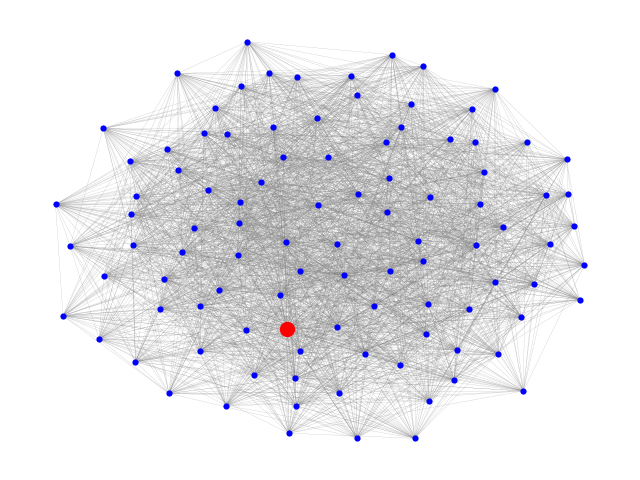
found node 73 with centrality 0.12598283530728402
Total running time of the script: (0 minutes 0.146 seconds)