
Tutorial#
This guide can help you start working with NetworkX.
Creating a graph#
Create an empty graph with no nodes and no edges.
import networkx as nx
G = nx.Graph()
By definition, a Graph is a collection of nodes (vertices) along with
identified pairs of nodes (called edges, links, etc). In NetworkX, nodes can
be any hashable object e.g., a text string, an image, an XML object,
another Graph, a customized node object, etc.
Note
Python’s None object is not allowed to be used as a node. It
determines whether optional function arguments have been assigned in many
functions.
Nodes#
The graph G can be grown in several ways. NetworkX includes many
graph generator functions and
facilities to read and write graphs in many formats.
To get started though we’ll look at simple manipulations. You can add one node
at a time,
G.add_node(1)
or add nodes from any iterable container, such as a list
G.add_nodes_from([2, 3])
You can also add nodes along with node
attributes if your container yields 2-tuples of the form
(node, node_attribute_dict):
G.add_nodes_from([(4, {"color": "red"}), (5, {"color": "green"})])
Node attributes are discussed further below.
Nodes from one graph can be incorporated into another:
H = nx.path_graph(10)
G.add_nodes_from(H)
G now contains the nodes of H as nodes of G.
In contrast, you could use the graph H as a node in G.
G.add_node(H)
The graph G now contains H as a node. This flexibility is very powerful as
it allows graphs of graphs, graphs of files, graphs of functions and much more.
It is worth thinking about how to structure your application so that the nodes
are useful entities. Of course you can always use a unique identifier in G
and have a separate dictionary keyed by identifier to the node information if
you prefer.
Note
You should not change the node object if the hash depends on its contents.
Edges#
G can also be grown by adding one edge at a time,
G.add_edge(1, 2)
e = (2, 3)
G.add_edge(*e)  # unpack edge tuple*
by adding a list of edges,
G.add_edges_from([(1, 2), (1, 3)])
or by adding any ebunch of edges. An ebunch is any iterable
container of edge-tuples. An edge-tuple can be a 2-tuple of nodes or a 3-tuple
with 2 nodes followed by an edge attribute dictionary, e.g.,
(2, 3, {'weight': 3.1415}). Edge attributes are discussed further
below.
G.add_edges_from(H.edges)
There are no complaints when adding existing nodes or edges. For example, after removing all nodes and edges,
G.clear()
we add new nodes/edges and NetworkX quietly ignores any that are already present.
G.add_edges_from([(1, 2), (1, 3)])
G.add_node(1)
G.add_edge(1, 2)
G.add_node("spam")        # adds node "spam"
G.add_nodes_from("spam")  # adds 4 nodes: 's', 'p', 'a', 'm'
G.add_edge(3, 'm')
At this stage the graph G consists of 8 nodes and 3 edges, as can be seen by:
G.number_of_nodes()
8
G.number_of_edges()
3
Note
The order of adjacency reporting (e.g., G.adj,
G.successors,
G.predecessors) is the order of
edge addition. However, the order of G.edges is the order of the adjacencies
which includes both the order of the nodes and each
node’s adjacencies. See example below:
DG = nx.DiGraph()
DG.add_edge(2, 1)   # adds the nodes in order 2, 1
DG.add_edge(1, 3)
DG.add_edge(2, 4)
DG.add_edge(1, 2)
assert list(DG.successors(2)) == [1, 4]
assert list(DG.edges) == [(2, 1), (2, 4), (1, 3), (1, 2)]
Examining elements of a graph#
We can examine the nodes and edges. Four basic graph properties facilitate
reporting: G.nodes, G.edges, G.adj and G.degree. These
are set-like views of the nodes, edges, neighbors (adjacencies), and degrees
of nodes in a graph. They offer a continually updated read-only view into
the graph structure. They are also dict-like in that you can look up node
and edge data attributes via the views and iterate with data attributes
using methods .items(), .data().
If you want a specific container type instead of a view, you can specify one.
Here we use lists, though sets, dicts, tuples and other containers may be
better in other contexts.
list(G.nodes)
[1, 2, 3, 'spam', 's', 'p', 'a', 'm']
list(G.edges)
[(1, 2), (1, 3), (3, 'm')]
list(G.adj[1]) # or list(G.neighbors(1))
[2, 3]
G.degree[1] # the number of edges incident to 1
2
One can specify to report the edges and degree from a subset of all nodes
using an nbunch. An nbunch is any of: None (meaning all nodes),
a node, or an iterable container of nodes that is not itself a node in the
graph.
G.edges([2, 'm'])
EdgeDataView([(2, 1), ('m', 3)])
G.degree([2, 3])
DegreeView({2: 1, 3: 2})
Access patterns#
Both nodes and edges can be accessed either as attributes, e.g. G.nodes or
G.edges, or as callables e.g. G.nodes() or G.edges().
The attribute-like access pattern is most convenient when setting/modifying node or
edge data:
G.nodes["spam"]["color"] = "blue"
G.edges[(1, 2)]["weight"] = 10
While the callable pattern is useful for inspecting node or edge attributes (and edge keys for multigraphs):
G.edges(data=True)
EdgeDataView([(1, 2, {'weight': 10}), (1, 3, {}), (3, 'm', {})])
G.nodes(data="color")
NodeDataView({1: None, 2: None, 3: None, 'spam': 'blue', 's': None, 'p': None, 'a': None, 'm': None}, data='color')
See the section on attributes for details.
Removing elements from a graph#
One can remove nodes and edges from the graph in a similar fashion to adding.
Use methods
Graph.remove_node(),
Graph.remove_nodes_from(),
Graph.remove_edge()
and
Graph.remove_edges_from().
Removing a node also removes its incident edges:
G.remove_node(2)
G.remove_nodes_from("spam")
list(G.nodes)
[1, 3, 'spam']
list(G.edges)
[(1, 3)]
Removing a specific edge only affects that edge:
G.remove_edge(1, 3)
list(G.nodes)
[1, 3, 'spam']
list(G.edges)
[]
Using the graph constructors#
Graph objects do not have to be built up incrementally - data specifying graph structure can be passed directly to the constructors of the various graph classes. When creating a graph structure by instantiating one of the graph classes you can specify data in several formats.
G.add_edge(1, 2)
H = nx.DiGraph(G)  # create a DiGraph using the connections from G
list(H.edges())
[(1, 2), (2, 1)]
edgelist = [(0, 1), (1, 2), (2, 3)]
H = nx.Graph(edgelist)  # create a graph from an edge list
list(H.edges())
[(0, 1), (1, 2), (2, 3)]
adjacency_dict = {0: (1, 2), 1: (0, 2), 2: (0, 1)}
H = nx.Graph(adjacency_dict)  # create a Graph dict mapping nodes to nbrs
list(H.edges())
[(0, 1), (0, 2), (1, 2)]
What to use as nodes and edges#
You might notice that nodes and edges are not specified as NetworkX
objects. This leaves you free to use meaningful items as nodes and
edges. The most common choices are numbers or strings, but a node can
be any hashable object (except None), and an edge can be associated
with any object x using G.add_edge(n1, n2, object=x).
As an example, n1 and n2 could be protein objects from the RCSB Protein
Data Bank, and x could refer to an XML record of publications detailing
experimental observations of their interaction.
We have found this power quite useful, but its abuse
can lead to surprising behavior unless one is familiar with Python.
If in doubt, consider using convert_node_labels_to_integers() to obtain
a more traditional graph with integer labels.
Accessing edges and neighbors#
In addition to the views Graph.edges, and Graph.adj,
access to edges and neighbors is possible using subscript notation.
G = nx.Graph([(1, 2, {"color": "yellow"})])
G[1]  # same as G.adj[1]
AtlasView({2: {'color': 'yellow'}})
G[1][2]
{'color': 'yellow'}
G.edges[1, 2]
{'color': 'yellow'}
You can get/set the attributes of an edge using subscript notation if the edge already exists.
G.add_edge(1, 3)
G[1][3]['color'] = "blue"
G.edges[1, 2]['color'] = "red"
G.edges[1, 2]
{'color': 'red'}
Fast examination of all (node, adjacency) pairs is achieved using
G.adjacency(), or G.adj.items().
Note that for undirected graphs, adjacency iteration sees each edge twice.
FG = nx.Graph()
FG.add_weighted_edges_from([(1, 2, 0.125), (1, 3, 0.75), (2, 4, 1.2), (3, 4, 0.375)])
for n, nbrs in FG.adj.items():
   for nbr, eattr in nbrs.items():
       wt = eattr['weight']
       if wt < 0.5: print(f"({n}, {nbr}, {wt:.3})")
(1, 2, 0.125)
(2, 1, 0.125)
(3, 4, 0.375)
(4, 3, 0.375)
Convenient access to all edges is achieved with the edges property.
for (u, v, wt) in FG.edges.data('weight'):
    if wt < 0.5:
        print(f"({u}, {v}, {wt:.3})")
(1, 2, 0.125)
(3, 4, 0.375)
Adding attributes to graphs, nodes, and edges#
Attributes such as weights, labels, colors, or whatever Python object you like, can be attached to graphs, nodes, or edges.
Each graph, node, and edge can hold key/value attribute pairs in an associated
attribute dictionary (the keys must be hashable). By default these are empty,
but attributes can be added or changed using add_edge, add_node or direct
manipulation of the attribute dictionaries named G.graph, G.nodes, and
G.edges for a graph G.
Graph attributes#
Assign graph attributes when creating a new graph
G = nx.Graph(day="Friday")
G.graph
{'day': 'Friday'}
Or you can modify attributes later
G.graph['day'] = "Monday"
G.graph
{'day': 'Monday'}
Node attributes#
Add node attributes using add_node(), add_nodes_from(), or G.nodes
G.add_node(1, time='5pm')
G.add_nodes_from([3], time='2pm')
G.nodes[1]
{'time': '5pm'}
G.nodes[1]['room'] = 714
G.nodes.data()
NodeDataView({1: {'time': '5pm', 'room': 714}, 3: {'time': '2pm'}})
Note that adding a node to G.nodes does not add it to the graph, use
G.add_node() to add new nodes. Similarly for edges.
Edge Attributes#
Add/change edge attributes using add_edge(), add_edges_from(),
or subscript notation.
G.add_edge(1, 2, weight=4.7 )
G.add_edges_from([(3, 4), (4, 5)], color='red')
G.add_edges_from([(1, 2, {'color': 'blue'}), (2, 3, {'weight': 8})])
G[1][2]['weight'] = 4.7
G.edges[3, 4]['weight'] = 4.2
The special attribute weight should be numeric as it is used by
algorithms requiring weighted edges.
Directed graphs#
The DiGraph class provides additional methods and properties specific
to directed edges, e.g.,
DiGraph.out_edges, DiGraph.in_degree,
DiGraph.predecessors(), DiGraph.successors() etc.
To allow algorithms to work with both classes easily, the directed versions of
neighbors is equivalent to
successors while DiGraph.degree reports the sum
of DiGraph.in_degree and DiGraph.out_degree even though that may
feel inconsistent at times.
DG = nx.DiGraph()
DG.add_weighted_edges_from([(1, 2, 0.5), (3, 1, 0.75)])
DG.out_degree(1, weight='weight')
0.5
DG.degree(1, weight='weight')
1.25
list(DG.successors(1))
[2]
list(DG.neighbors(1))
[2]
Some algorithms work only for directed graphs and others are not well
defined for directed graphs. Indeed the tendency to lump directed
and undirected graphs together is dangerous. If you want to treat
a directed graph as undirected for some measurement you should probably
convert it using Graph.to_undirected() or with
H = nx.Graph(G) # create an undirected graph H from a directed graph G
Multigraphs#
NetworkX provides classes for graphs which allow multiple edges
between any pair of nodes. The MultiGraph and
MultiDiGraph
classes allow you to add the same edge twice, possibly with different
edge data. This can be powerful for some applications, but many
algorithms are not well defined on such graphs.
Where results are well defined,
e.g., MultiGraph.degree() we provide the function. Otherwise you
should convert to a standard graph in a way that makes the measurement
well defined.
MG = nx.MultiGraph()
MG.add_weighted_edges_from([(1, 2, 0.5), (1, 2, 0.75), (2, 3, 0.5)])
dict(MG.degree(weight='weight'))
{1: 1.25, 2: 1.75, 3: 0.5}
GG = nx.Graph()
for n, nbrs in MG.adjacency():
   for nbr, edict in nbrs.items():
       minvalue = min([d['weight'] for d in edict.values()])
       GG.add_edge(n, nbr, weight = minvalue)

nx.shortest_path(GG, 1, 3)
[1, 2, 3]
Graph generators and graph operations#
In addition to constructing graphs node-by-node or edge-by-edge, they can also be generated by
1. Applying classic graph operations, such as:#
|
Returns the subgraph induced on nodes in nbunch. |
|
Combine graphs G and H. |
|
Combine graphs G and H. |
|
Returns the Cartesian product of G and H. |
|
Compose graph G with H by combining nodes and edges into a single graph. |
|
Returns the graph complement of G. |
|
Returns a copy of the graph G with all of the edges removed. |
|
Returns an undirected view of the graph |
|
Returns a directed view of the graph |
2. Using a call to one of the classic small graphs, e.g.,#
|
Returns the Petersen Graph. |
|
Returns the Tutte graph. |
|
Return a small maze with a cycle. |
|
Returns the 3-regular Platonic Tetrahedral graph. |
3. Using a (constructive) generator for a classic graph, e.g.,#
|
Return the complete graph |
|
Returns the complete bipartite graph |
|
Returns the Barbell Graph: two complete graphs connected by a path. |
|
Returns the Lollipop Graph; |
like so:
K_5 = nx.complete_graph(5)
K_3_5 = nx.complete_bipartite_graph(3, 5)
barbell = nx.barbell_graph(10, 10)
lollipop = nx.lollipop_graph(10, 20)
4. Using a stochastic graph generator, e.g,#
|
Returns a \(G_{n,p}\) random graph, also known as an Erdős-Rényi graph or a binomial graph. |
|
Returns a Watts–Strogatz small-world graph. |
|
Returns a random graph using Barabási–Albert preferential attachment |
|
Returns a random lobster graph. |
like so:
er = nx.erdos_renyi_graph(100, 0.15)
ws = nx.watts_strogatz_graph(30, 3, 0.1)
ba = nx.barabasi_albert_graph(100, 5)
red = nx.random_lobster_graph(100, 0.9, 0.9)
5. Reading a graph stored in a file using common graph formats#
NetworkX supports many popular formats, such as edge lists, adjacency lists, GML, GraphML, LEDA and others.
nx.write_gml(red, "path.to.file")
mygraph = nx.read_gml("path.to.file")
For details on graph formats see Reading and writing graphs and for graph generator functions see Graph generators
Analyzing graphs#
The structure of G can be analyzed using various graph-theoretic
functions such as:
G = nx.Graph()
G.add_edges_from([(1, 2), (1, 3)])
G.add_node("spam")       # adds node "spam"
list(nx.connected_components(G))
[{1, 2, 3}, {'spam'}]
sorted(d for n, d in G.degree())
[0, 1, 1, 2]
nx.clustering(G)
{1: 0, 2: 0, 3: 0, 'spam': 0}
Some functions with large output iterate over (node, value) 2-tuples.
These are easily stored in a dict structure if you desire.
sp = dict(nx.all_pairs_shortest_path(G))
sp[3]
{3: [3], 1: [3, 1], 2: [3, 1, 2]}
See Algorithms for details on graph algorithms supported.
Floating point considerations#
Many NetworkX algorithms work with numeric values, such as edge weights. Once your input contains floating point numbers, all results are inherently approximate due to the limited precision of floating point arithmetic. This is especially true for algorithms such as shortest-path, flows, cuts, minimum-spanning, etc. Basically any time a min or max value is computed.
For example:
import networkx as nx

tiny = 5e-17

G = nx.DiGraph()
G.add_edge('A', 'B', weight=0.1)
G.add_edge('B', 'C', weight=0.1)
G.add_edge('C', 'D', weight=0.1)
G.add_edge('A', 'D', weight=0.3 + tiny)

path = nx.shortest_path(G, source='A', target='D', weight='weight')
print(path)
['A', 'D']
Even though A -> B -> C -> D has a total weight of 0.3, the direct edge
A -> D with 0.3 + 1e-17 is selected. This demonstrates that algorithms
treat floating point numbers as exact, so very small differences can change the
outcome.
Floating point arithmetic can produce unintuitive results because certain
values, such as 0.3, cannot be represented exactly in binary. For example:
0.1 + 0.1 + 0.1 > 0.3
True
In general, when using floating point numbers in NetworkX, you should expect results to be approximate rather than exact. Multiplying weights by a large number and converting them to integers can help reduce some subtle comparison issues, but it does not fully eliminate them. NetworkX does not automatically apply tolerances in numeric comparisons.
Below is a version of the previous example using the recommended technique with different precision tolerances.
for precision in [16, 17]:
    path = nx.shortest_path(
        G,
        source='A',
        target='D',
        weight=lambda u, v, d: int(d['weight'] * 10 ** precision)
    )
    print(f"With {precision} precision digits, path is {path}")
With 16 precision digits, path is ['A', 'D']
With 17 precision digits, path is ['A', 'B', 'C', 'D']
Using NetworkX backends#
NetworkX can be configured to use separate third-party backends to improve performance and add functionality. Backends are optional, installed separately, and can be enabled either directly in the user’s code or through environment variables.
Several backends are available to accelerate NetworkX–often significantly–using GPUs, parallel processing, and other optimizations, while other backends add additional features such as graph database integration. Multiple backends can be used together to compose a NetworkX runtime environment optimized for a particular system or use case.
Note
Refer to the Backends section to see a list of available backends known to work with the current stable release of NetworkX.
NetworkX uses backends by dispatching function calls at runtime to corresponding functions provided by backends, either automatically via configuration variables, or explicitly by hard-coded arguments to functions.
Automatic dispatch#
Automatic dispatch is possibly the easiest and least intrusive means by which a user can use backends with NetworkX code. This technique is useful for users that want to write portable code that runs on systems without specific backends, or simply want to use backends for existing code without modifications.
The example below configures NetworkX to automatically dispatch to a backend
named fast_backend for all NetworkX functions that fast_backend supports.
If
fast_backenddoes not support a NetworkX function used by the application, the default NetworkX implementation for that function will be used.If
fast_backendis not installed on the system running this code, an exception will be raised.
bash$> NETWORKX_BACKEND_PRIORITY=fast_backend python my_script.py
import networkx as nx
G = nx.karate_club_graph()
pr = nx.pagerank(G)  # runs using backend from NETWORKX_BACKEND_PRIORITY, if set
The equivalent configuration can be applied to NetworkX directly to the code
through the NetworkX config global parameters, which may be useful if
environment variables are not suitable. This will override the corresponding
environment variable allowing backends to be enabled programmatically in Python
code. However, the tradeoff is slightly less portability as updating the
backend specification may require a small code change instead of simply
updating an environment variable.
nx.config.backend_priority = ["fast_backend"]
pr = nx.pagerank(G)
Automatic dispatch using the NETWORKX_BACKEND_PRIORITY environment variable
or the nx.config.backend_priority global config also allows for the
specification of multiple backends, ordered based on the priority which
NetworkX should attempt to dispatch to.
The following examples both configure NetworkX to dispatch functions first to
fast_backend if it supports the function, then other_backend if
fast_backend does not, then finally the default NetworkX implementation if no
backend specified can handle the call.
bash$> NETWORKX_BACKEND_PRIORITY="fast_backend,other_backend" python my_script.py
nx.config.backend_priority = ["fast_backend", "other_backend"]
Tip
NetworkX includes debug logging calls using Python’s standard logging mechanism. These can be enabled to help users understand when and how backends are being used.
To enable debug logging only in NetworkX modules:
import logging
_l = logging.getLogger("networkx")
_l.addHandler(_h:=logging.StreamHandler())
_h.setFormatter(logging.Formatter("%(levelname)s:NetworkX:%(message)s"))
_l.setLevel(logging.DEBUG)
or to enable it globally:
logging.basicConfig(level=logging.DEBUG)
Explicit dispatch#
Backends can also be used explicitly on a per-function call basis by specifying
a backend using the backend= keyword argument. This technique not only
requires that the backend is installed, but also requires that the backend
implement the function, since NetworkX will not fall back to the default NetworkX
implementation if a backend is specified with backend=.
This is possibly the least portable option, but has the advantage that NetworkX
will raise an exception if fast_backend cannot be used, which is useful for
users that require a specific implementation. Explicit dispatch can also
provide a more interactive experience and is especially useful for
demonstrations, experimentation, and debugging.
pr = nx.pagerank(G, backend="fast_backend")
Advanced dispatching options#
The NetworkX dispatcher allows users to use backends for NetworkX code in very specific ways not covered in this tutorial. Refer to the Backends reference section for details on topics such as:
Control of how specific function types (algorithms vs. generators) are dispatched to specific backends
Details on automatic conversions to/from backend and NetworkX graphs for dispatch and fallback
Caching graph conversions
Explicit backend graph instantiation and dispatching based on backend graph types
and more…
Drawing graphs#
NetworkX is not primarily a graph drawing package but basic drawing with Matplotlib as well as an interface to use the open source Graphviz software package are included. These are part of the networkx.drawing module and will be imported if possible.
First import Matplotlib’s plot interface (pylab works too)
import matplotlib.pyplot as plt
To test if the import of ~networkx.drawing.nx_pylab was successful draw G
using one of
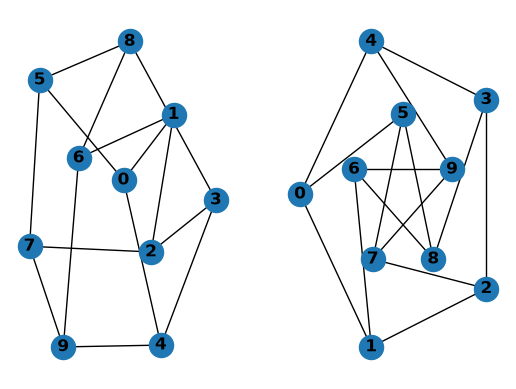
G = nx.petersen_graph()
subax1 = plt.subplot(121)
nx.draw(G, with_labels=True, font_weight='bold')
subax2 = plt.subplot(122)
nx.draw_shell(G, nlist=[range(5, 10), range(5)], with_labels=True, font_weight='bold')
when drawing to an interactive display. Note that you may need to issue a Matplotlib
plt.show()
command if you are not using matplotlib in interactive mode.
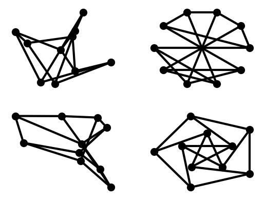
options = {
    'node_color': 'black',
    'node_size': 100,
    'width': 3,
}
subax1 = plt.subplot(221)
nx.draw_random(G, **options)
subax2 = plt.subplot(222)
nx.draw_circular(G, **options)
subax3 = plt.subplot(223)
nx.draw_spectral(G, **options)
subax4 = plt.subplot(224)
nx.draw_shell(G, nlist=[range(5,10), range(5)], **options)
You can find additional options via draw_networkx() and
layouts via the layout module.
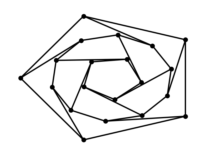
You can use multiple shells with draw_shell().
G = nx.dodecahedral_graph()
shells = [[2, 3, 4, 5, 6], [8, 1, 0, 19, 18, 17, 16, 15, 14, 7], [9, 10, 11, 12, 13]]
nx.draw_shell(G, nlist=shells, **options)
To save drawings to a file, use, for example
>>> nx.draw(G)
>>> plt.savefig("path.png")
This function writes to the file path.png in the local directory. If Graphviz and
PyGraphviz or pydot, are available on your system, you can also use
networkx.drawing.nx_agraph.graphviz_layout or
networkx.drawing.nx_pydot.graphviz_layout to get the node positions, or write
the graph in dot format for further processing.
>>> from networkx.drawing.nx_pydot import write_dot
>>> pos = nx.nx_agraph.graphviz_layout(G)
>>> nx.draw(G, pos=pos)
>>> write_dot(G, 'file.dot')
See Drawing for additional details.
NX-Guides#
If you are interested in learning more about NetworkX, graph theory and network analysis then you should check out nx-guides. There you can find tutorials, real-world applications and in-depth examinations of graphs and network algorithms. All the material is official and was developed and curated by the NetworkX community.