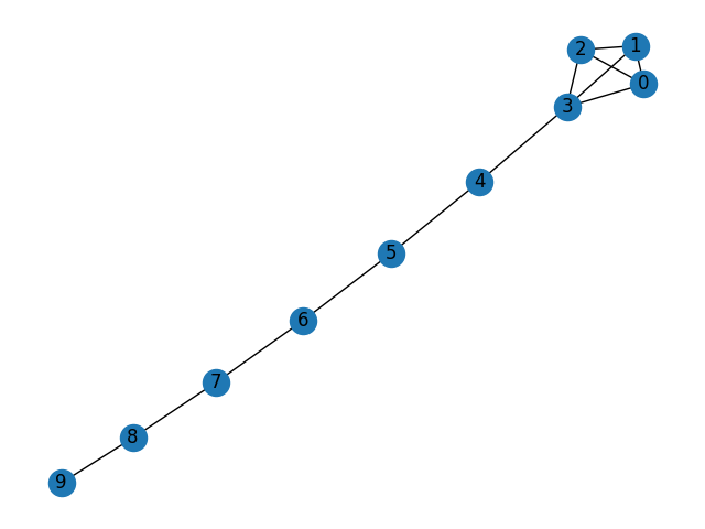
Properties

Compute some network properties for the lollipop graph.

from collections import Counter
import itertools
import matplotlib.pyplot as plt
import networkx as nx
from pprint import pprint

G = nx.lollipop_graph(4, 6)

A quick summary of basic properties is available via nx.describe

nx.describe(G)
print(f"density: {nx.density(G)}")

print("\nShortest path length between all node pairs:")
print("  {source node: {target node: path length}")
path_lengths = dict(nx.all_pairs_shortest_path_length(G))
pprint(path_lengths)

print(f"\naverage shortest path length {nx.average_shortest_path_length(G)}")

Number of nodes                : 10
Number of edges                : 12
Directed                       : False
Multigraph                     : False
Tree                           : False
Bipartite                      : False
Average degree (min, max)      : 2.40 (1, 4)
Number of connected components : 1
Density                        : 0.26666666666666666
density: 0.26666666666666666

Shortest path length between all node pairs:
  {source node: {target node: path length}
{0: {0: 0, 1: 1, 2: 1, 3: 1, 4: 2, 5: 3, 6: 4, 7: 5, 8: 6, 9: 7},
 1: {0: 1, 1: 0, 2: 1, 3: 1, 4: 2, 5: 3, 6: 4, 7: 5, 8: 6, 9: 7},
 2: {0: 1, 1: 1, 2: 0, 3: 1, 4: 2, 5: 3, 6: 4, 7: 5, 8: 6, 9: 7},
 3: {0: 1, 1: 1, 2: 1, 3: 0, 4: 1, 5: 2, 6: 3, 7: 4, 8: 5, 9: 6},
 4: {0: 2, 1: 2, 2: 2, 3: 1, 4: 0, 5: 1, 6: 2, 7: 3, 8: 4, 9: 5},
 5: {0: 3, 1: 3, 2: 3, 3: 2, 4: 1, 5: 0, 6: 1, 7: 2, 8: 3, 9: 4},
 6: {0: 4, 1: 4, 2: 4, 3: 3, 4: 2, 5: 1, 6: 0, 7: 1, 8: 2, 9: 3},
 7: {0: 5, 1: 5, 2: 5, 3: 4, 4: 3, 5: 2, 6: 1, 7: 0, 8: 1, 9: 2},
 8: {0: 6, 1: 6, 2: 6, 3: 5, 4: 4, 5: 3, 6: 2, 7: 1, 8: 0, 9: 1},
 9: {0: 7, 1: 7, 2: 7, 3: 6, 4: 5, 5: 4, 6: 3, 7: 2, 8: 1, 9: 0}}

average shortest path length 3.1777777777777776

Histogram of path lengths - note that this counts each path twice: from src -> tgt and tgt -> src.

print("\nDistribution of shortest path lengths")
path_length_distribution = Counter(
    itertools.chain.from_iterable(t.values() for t in path_lengths.values())
)
pprint({pl: num // 2 for pl, num in path_length_distribution.items()})

Distribution of shortest path lengths
{0: 5, 1: 12, 2: 8, 3: 7, 4: 6, 5: 5, 6: 4, 7: 3}

Basic distance measures. In some cases it is possible to pass in pre-computed eccentricity values to speed up subsequent computations. Re-using computed values may significantly improve computation times for larger graphs

eccentricity = nx.eccentricity(G)
print(f"\neccentricity: {eccentricity}")
print(f"radius: {nx.radius(G, e=eccentricity)}")
print(f"diameter: {nx.diameter(G, e=eccentricity)}")
print(f"center: {nx.center(G, e=eccentricity)}")
print(f"periphery: {nx.periphery(G, e=eccentricity)}")

pos = nx.spring_layout(G, seed=3068)  # Seed layout for reproducibility
nx.draw(G, pos=pos, with_labels=True)
plt.show()

eccentricity: {0: 7, 1: 7, 2: 7, 3: 6, 4: 5, 5: 4, 6: 4, 7: 5, 8: 6, 9: 7}
radius: 4
diameter: 7
center: [5, 6]
periphery: [0, 1, 2, 9]